Linear Algebra & Geometry of the Perceptron

Perceptrons are one of the simplest forms of artificial neural networks, but they are far more than simple computational models. They are geometric and algebraic machines that classify data by creating boundaries in space. Understanding the linear algebra and geometry behind perceptrons helps us see why they succeed in some tasks and fail in others. This module explores these concepts step by step, combining algebraic formulations with geometric intuition.

Representing Inputs & Weights as Vectors

A perceptron makes decisions by weighing input features. To describe its behavior mathematically, we treat both inputs and weights as vectors, which allows us to use tools from linear algebra, such as dot products, scalar multiplication, and vector addition.

Input vector

All features of a single data point are collected into a vector. For a point with three features x1, x2, x3, the input vector is:

x = [x1, x2, x3]

Each element represents a measurable property, such as pixel intensity, temperature, or other numeric value. Representing inputs as vectors lets us compute alignment and direction in space, which is essential for classification.

Weight vector

Each input has a corresponding weight in the perceptron:

w = [w1, w2, w3]

Weights determine how important each feature is in making the final decision. Larger weights increase a feature’s influence, while smaller or negative weights reduce or reverse it.

Computing the Weighted Sum

The perceptron combines the inputs using a weighted sum, which in linear algebra is expressed as a dot product:

weighted sum = w1x1 + w2x2 + w3x3 = w · x

A positive dot product indicates that the input vector points roughly in the same direction as the weight vector, suggesting the positive class, while a negative dot product indicates the input points in the opposite direction, suggesting the negative class.

Defining Decision Boundaries with Hyperplanes

A perceptron classifies points by creating a decision boundary that separates the positive and negative classes. Mathematically, this boundary is defined by the hyperplane equation:

w · x = 0

In 2D, the hyperplane appears as a line, in 3D it is a plane, and in higher dimensions it is called a hyperplane. The weight vector w is perpendicular to the hyperplane. Points on one side of the hyperplane are classified as positive, while points on the other side are classified as negative. Adjusting the weights rotates the hyperplane around the origin.

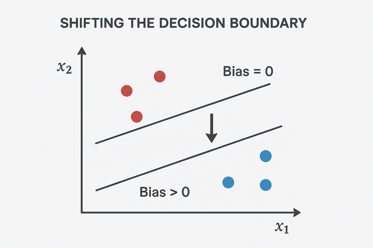
Introducing Bias for Flexibility

To give the perceptron more flexibility, we add a bias term b to the weighted sum:

w · x + b

The bias shifts the hyperplane without rotating it. Without a bias, the hyperplane must pass through the origin, which limits its ability to separate some datasets.

Decision rule:

• If w · x + b ≥ 0 → output = 1 (positive class)
• If w · x + b < 0 → output = 0 (negative class)

Understanding Linear Separability

A dataset is linearly separable if there exists a hyperplane that perfectly divides the classes. Mathematically:

• For all positive points: w · x + b ≥ 0
• For all negative points: w · x + b < 0

If no such hyperplane exists, a single-layer perceptron cannot perfectly classify the data.

Convex Sets

The convex hull of a set of points is the smallest convex set that contains all points in the set. A set is convex if the line segment connecting any two points in the set lies entirely within the set.

Relationship to Linear Separability

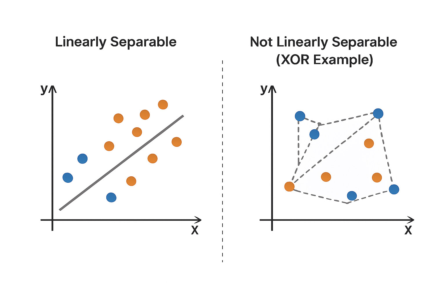
Two classes are linearly separable if and only if their convex hulls are disjoint (do not intersect). If the convex hulls overlap, no single hyperplane can separate the classes perfectly.

Updating Weights: Correcting Misclassifications

When a perceptron misclassifies a point, it updates its weights using the following learning rule:

w = w + learning_rate * (target - output) * x

• If a negative point is misclassified as positive, the weight vector moves away from the point to correct the error.
• If a positive point is misclassified as negative, the weight vector moves toward the point to increase alignment and correct the mistake.

Convergence of the Perceptron Algorithm

If the dataset is linearly separable, the perceptron is guaranteed to converge after a finite number of updates.

Reasoning:

• Assume there exists an ideal weight vector w* that perfectly separates the classes.
• Each weight update increases the alignment (dot product) between w and w*.
• The length of w grows at a limited rate due to vector addition properties.

These facts guarantee that the algorithm finds a solution in finite steps, making perceptrons reliable for linearly separable problems.